Step 1: create synthetic data (or load your own data)
In this post for demonstration purposes I will generate very simple dataset for visualization purposes. To do so, I will use numpy’s multivariate gaussian function to generate some data.
# import some packages
import numpy as np
import matplotlib.pyplot as plt

# generate 5000 2-dimensional gaussian distributed data points
# with high variance on the main diagonal
mean = [0, 0]
covariance = [[10, 5], [5, 5]]
x, y = np.random.multivariate_normal(mean, covariance, 5000).T
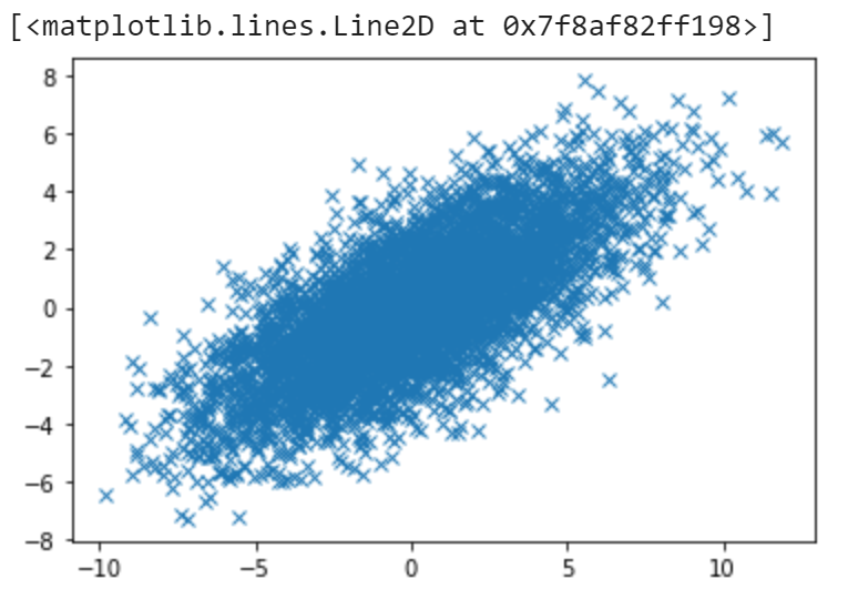
plt.plot(x, y, 'x')
# put x, y's into a design matrix.
X = [[x[i], y[i]] for i in range(len(x))]
X = np.asarray(X)
We now have the following data:

Step 2: Standardization (or normalization)
second step is to standardize data. This just means we want in every dimension data has mean of 0 and variance of 1. The reason we do this is because PCA is sensitive to scale. For example, when one feature’s values are like 1, 2, 3 and another feature’s values are 1000, 1005, 1010. This situation will mess up PCA. In python this is pretty easy. We can just do
from sklearn.preprocessing import StandardScaler
X = StandardScaler().fit_transform(X)
step 3: SVD or eigendecomposition on covariance matrix:
This is the most interesting step that the real computation happens. SVD on original $X$ matrix and eigendecomposition on $X^{T}X$ are equivalent. We will choose to do SVD. In python SVD is just one line of code:
# s is the singular values (sqrt(eigenvalues)).
u, s, v = np.linalg.svd(X)
And now we have s which contains all the square root of eigenvalues of $X^{T}X$.
step 4: pick the largest m eigenvalues:
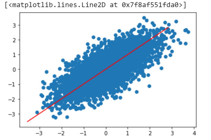
In our example $s = [92.81428825, 37.2224112]$, and here I will choose the first eigenvector because it has the largest eigenvalue. We can plot the eigenspace to see if it matches our intuition:
plt.scatter(X[:,0], X[:,1])
x = [v[0,:][0] * i for i in range(-5,5)]
y = [v[0,:][1] * i for i in range(-5,5)]
plt.plot(x, y, color = 'r')

We can see that the red line is the projected space, which is the axis with most variation. This looks good
step 5: project original dataset into eigenspace using the eigenvectors we found:
In this step we simply transfrom the original dataset use the eigenvector we found.
# select the first eigenvector in eigenvector matrix v,
# since the first eigenvector has the greatest eigenvalue.
eigenVector = v[0,:].reshape(-1,1)
# @ is matrix multiplication in numpy.
dimensionReducedData = X @ eigenVector
Now we are done! the dimensionReducedData will consist of 5000 rows but only 1 column!
conclusion
In real machine learning projects we don’t need to do these tedious things. We just need to call the PCA algorithm on sklearn library. The above algorithm just demonstrates that PCA is nothing but eigendecomposition with covariance matrix of the data. Underlying idea is really simple and easy to implement.